Loading Packages
## Warning: package 'tidyverse' was built under R version 4.3.3
## Warning: package 'ggplot2' was built under R version 4.3.3
## Warning: package 'lubridate' was built under R version 4.3.3
## ── Attaching core tidyverse packages ──────────────── tidyverse 2.0.0 ──
## ✔ dplyr     1.1.4     ✔ readr     2.1.5
## ✔ forcats   1.0.0     ✔ stringr   1.5.1
## ✔ ggplot2   3.5.1     ✔ tibble    3.2.1
## ✔ lubridate 1.9.4     ✔ tidyr     1.3.1
## ✔ purrr     1.0.2
## ── Conflicts ────────────────────────────────── tidyverse_conflicts() ──
## ✖ dplyr::filter() masks stats::filter()
## ✖ dplyr::lag()    masks stats::lag()
## ℹ Use the conflicted package (<http://conflicted.r-lib.org/>) to force all conflicts to become errors
## Warning: package 'ggthemes' was built under R version 4.3.3
## Warning: package 'ggridges' was built under R version 4.3.3
## Warning: package 'treemapify' was built under R version 4.3.3
## Warning: package 'waffle' was built under R version 4.3.3
## Warning: package 'patchwork' was built under R version 4.3.3
## Warning: package 'cowplot' was built under R version 4.3.3
##
## Attaching package: 'cowplot'
##
## The following object is masked from 'package:patchwork':
##
##     align_plots
##
## The following object is masked from 'package:ggthemes':
##
##     theme_map
##
## The following object is masked from 'package:lubridate':
##
##     stamp
Load Data from GitHub
founder <- read_csv("https://raw.githubusercontent.com/rfordatascience/tidytuesday/master/data/2023/2023-04-18/founder_crops.csv")
## Rows: 4490 Columns: 24
## ── Column specification ────────────────────────────────────────────────
## Delimiter: ","
## chr (18): source, source_id, source_site_name, site_name, phase, phase_descr...
## dbl  (6): latitude, longitude, age_start, age_end, n, prop
##
## ℹ Use `spec()` to retrieve the full column specification for this data.
## ℹ Specify the column types or set `show_col_types = FALSE` to quiet this message.
## Rows: 4,490
## Columns: 24
## $ source            <chr> "ORIGINS", "ORIGINS", "ORIGINS", "ORIGINS", "ORIGINS…
## $ source_id         <chr> "16433–16433", "12007–12249", "12013–12298", "11956–…
## $ source_site_name  <chr> "Ayn Abu Nukhayla", "Abu Hureyra", "Abu Hureyra", "A…
## $ site_name         <chr> "Ayn Abu Nakhayla", "Abu Hureyra", "Abu Hureyra", "A…
## $ latitude          <dbl> 29.84, 35.87, 35.87, 35.87, 35.87, 35.87, 35.87, 35.…
## $ longitude         <dbl> 35.24, 38.40, 38.40, 38.40, 38.40, 38.40, 38.40, 38.…
## $ phase             <chr> "PPNB", "Abu Hureyra 1 (epipalaeolithic) phase 1", "…
## $ phase_description <chr> NA, "Dates approximated from Colledge & Conolly 2010…
## $ phase_code        <chr> "AANU PPNB", "ABHU Epip1", "ABHU Epip1", "ABHU Epip1…
## $ age_start         <dbl> 9578, 13096, 13096, 13096, 13096, 13096, 13096, 1309…
## $ age_end           <dbl> 9401, 12984, 12984, 12984, 12984, 12984, 12984, 1298…
## $ taxon_source      <chr> "Gypsophila", "Alyssum", "Arenaria serpyllifolia", "…
## $ n                 <dbl> 1, 6, 18, 184, 21, 15, 12, 42, 3, 3, 3, 6, 22, 234, …
## $ prop              <dbl> 0.5000000000, 0.0010398614, 0.0031195841, 0.03188908…
## $ reference         <chr> "HenryEtal03", "MooreEtal2000", "MooreEtal2000", "Mo…
## $ taxon_detail      <chr> "Gypsophila sp.", "Alyssum sp.", "Arenaria serpyllif…
## $ taxon             <chr> "Gypsophila spp. (incl. elegans, obionica, pilosa)",…
## $ genus             <chr> "Gypsophila", "Alyssum", "Arenaria", "Arnebia", "Arn…
## $ family            <chr> "Caryophillaceae", "Brassicaceae", "Caryophyllaceae"…
## $ category          <chr> "Wild plants", "Wild plants", "Wild plants", "Wild p…
## $ founder_crop      <chr> NA, NA, NA, NA, NA, NA, NA, NA, NA, NA, NA, NA, NA, …
## $ edibility         <chr> NA, NA, NA, NA, NA, "stems", "rhizomes, stems and le…
## $ grass_type        <chr> NA, NA, NA, NA, NA, NA, NA, NA, "Large/medium-seeded…
## $ legume_type       <chr> NA, NA, NA, NA, NA, NA, NA, NA, NA, NA, NA, NA, NA, …
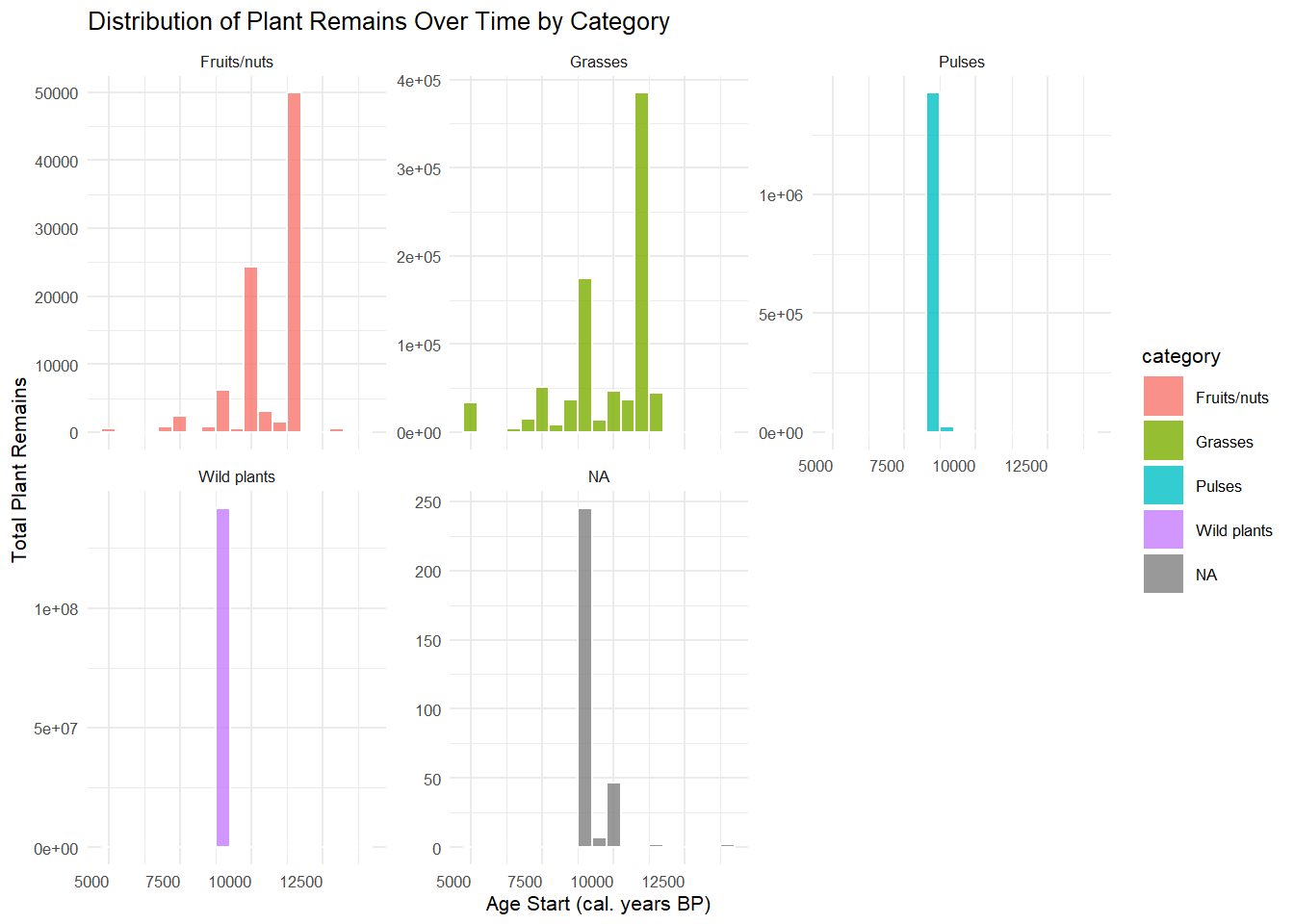
2. Histogram – Distribution of Plant Remains Over Time by
Category
p2 <- ggplot(founder, aes(x = age_start, weight = n, fill = category)) +
  geom_histogram(binwidth = 500, alpha = 0.8, color = "white") +
  facet_wrap(~ category, scales = "free_y") +
  theme_minimal(base_size = 8) +
  theme(
    axis.text.x = element_text(angle = 0, hjust = 1)
  ) +
  labs(
    title = "Distribution of Plant Remains Over Time by Category",
    x = "Age Start (cal. years BP)",
    y = "Total Plant Remains"
  )

p2
ggsave("plot2_histogram.png", plot = p2, width = 10, height = 6, dpi = 300)